PaperPlotR is designed for scientific figure workflows
that rely on ggplot2, but need additional structure around
styling, figure sizing, semantic colors, layout, and export.
The package aims to standardize repeated plotting decisions without
hiding the underlying ggplot2 workflow.
Inspect Available Presets
available_fig_specs()
#> [1] "2x2"     "2.58x2"  "4.9x2"   "4.9x4.9" "4.9"
available_journal_presets()
#> [1] "cell"   "nature" "ncomms"
available_output_presets()
#> [1] "cell"        "cell_half"   "nature"      "nature_half" "ncomms"
#> [6] "ncomms_half"
available_group_dictionaries()
#> [1] "default"
available_group_dictionaries(include_examples = TRUE)
#> [1] "default"                     "quinoa_samples"
#> [3] "subgenome_classes"           "trash_monomers"
#> [5] "trash_monomers_graphpad_alt" "ancestry_components"
Figure Size Helpers
fig_specs stores the built-in panel definitions used by
get_fig_size_cm() and panel_size().
fig_specs
#>      spec panel_w_cm panel_h_cm nonpanel_w_cm nonpanel_h_cm gap_cm base_font_pt
#> 1     2x2       2.00        2.0           0.9           0.9   0.15            7
#> 2  2.58x2       2.58        2.0           0.9           0.9   0.15            7
#> 3   4.9x2       4.90        2.0           0.9           0.9   0.15            7
#> 4 4.9x4.9       4.90        4.9           0.9           0.9   0.15            7
#>   min_linewidth
#> 1          0.35
#> 2          0.35
#> 3          0.35
#> 4          0.35
get_fig_size_cm("4.9x2", ncol = 3, nrow = 1)
#> $spec
#> [1] "4.9x2"
#>
#> $width_cm
#> [1] 15.9
#>
#> $height_cm
#> [1] 2.9
journal_preset("cell")
#> $journal
#> [1] "cell"
#>
#> $figure_width_cm
#> [1] 17.4
#>
#> $base_size_pt
#> [1] 8
#>
#> $min_text_pt
#> [1] 6
#>
#> $dpi
#> [1] 600
#>
#> $base_family
#> [1] "Arial"
#>
#> $line_width
#> [1] 0.4
recommend_panel_spec(n_panels = 4)
#> $n_panels
#> [1] 4
#>
#> $plot_type
#> [1] "general"
#>
#> $complexity
#> [1] "simple"
#>
#> $spec
#> [1] "4.9x4.9"
#>
#> $ncol
#> [1] 2
#>
#> $nrow
#> [1] 2
#>
#> $figure_width_cm
#> [1] 10.85
#>
#> $figure_height_cm
#> [1] 10.85
#>
#> $split_figure
#> [1] FALSE
#>
#> $rationale
#> [1] "Default main-figure rule keeps 1-6 panels at 4.9x4.9 for readable paper panels."
For dense figures, recommend_panel_spec() can suggest a
starting layout and indicate when splitting a figure is likely to be
clearer.
recommend_panel_spec(
  n_panels = 8,
  heatmap = TRUE,
  rotated_x_labels = TRUE,
  complex_legend = TRUE
)
#> $n_panels
#> [1] 8
#>
#> $plot_type
#> [1] "general"
#>
#> $complexity
#> [1] "complex"
#>
#> $spec
#> [1] "4.9x4.9"
#>
#> $ncol
#> [1] 4
#>
#> $nrow
#> [1] 2
#>
#> $figure_width_cm
#> [1] 20.95
#>
#> $figure_height_cm
#> [1] 10.85
#>
#> $split_figure
#> [1] TRUE
#>
#> $rationale
#> [1] "Panel count enters the small-multiples range, so the baseline recommendation starts from 2.58x2. Readability risks promote the layout to 4.9x4.9. The panel count and complexity suggest splitting the figure instead of forcing every panel into one page."
You can extend the defaults at runtime with custom registrations.
register_fig_spec(
  name = "6x4",
  panel_w_cm = 6,
  panel_h_cm = 4,
  layout_hint = "Wide single-panel figures"
)

register_palette(
  name = "study_palette",
  values = c("#1B3A57", "#2E6F95", "#58A4B0")
)

tail(available_fig_specs(), 1)
#> [1] "4.9"
tail(available_lab_palettes(), 1)
#> [1] "study_palette"
Theme and Color Scales
p <- ggplot(mtcars, aes(wt, mpg, colour = factor(cyl))) +
  geom_point(size = 2.2) +
  scale_color_lab() +
  theme_lab()

p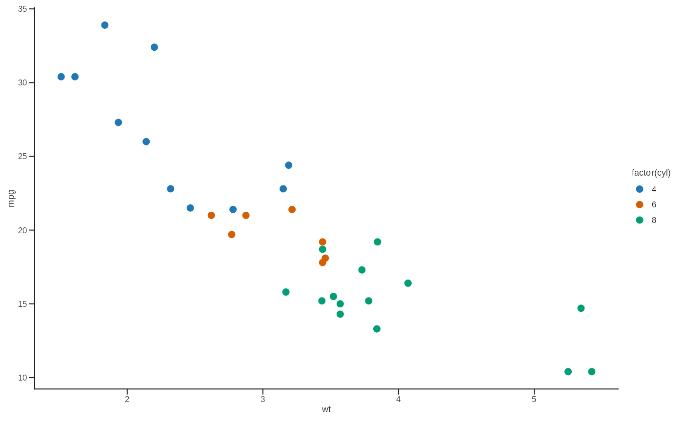
Use semantic group mappings when category names should keep consistent colors across plots.
group_colors("default")[1:4]
#>   Control Treatment        WT    Mutant
#> "#4D4D4D" "#D55E00" "#1F77B4" "#CC79A7"
The default dictionary is intentionally generic. Domain-specific dictionaries used in examples remain available for backward compatibility, but production projects should usually register their own semantic mapping.
register_group_dictionary(
  name = "experiment_groups",
  values = c(Control = "#4D4D4D", Treatment = "#D55E00", Rescue = "#009E73")
)

group_colors("experiment_groups")
#>   Control Treatment    Rescue
#> "#4D4D4D" "#D55E00" "#009E73"
Layout and Export
p1 <- ggplot(mtcars, aes(wt, mpg)) + geom_point() + theme_lab()
p2 <- ggplot(mtcars, aes(factor(cyl), mpg)) + geom_boxplot() + theme_lab()

layout_lab(p1, p2, ncol = 2)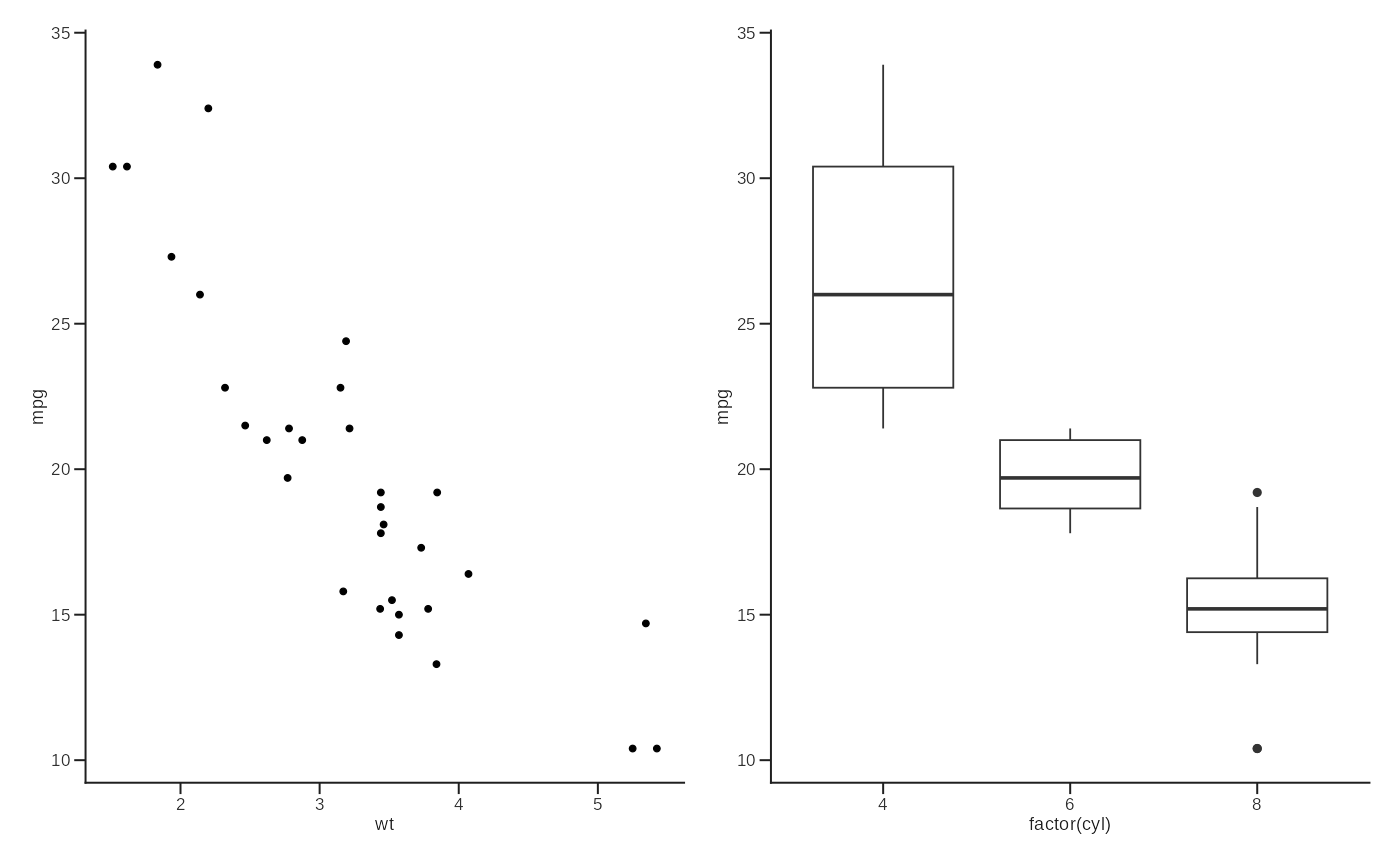
Use save_lab() when you want figure size to follow a
named panel spec plus a journal preset.
save_lab(
  plot = p1,
  filename = "figures/scatter_cell.png",
  spec = "4.9x4.9",
  journal = "cell",
  device = "ragg_png"
)
Use save_lab_plot() when you prefer named output presets
or direct width and height control.
Optional devices include "ragg_png",
"ragg_tiff", "svglite", and
"quartz_pdf" on macOS. Saved files are checked by default;
tune min_output_size_bytes or use
validate_output = FALSE for very small diagnostic
graphics.
Comparison Plots
PaperPlotR also provides lightweight wrappers for common
grouped comparison plots.
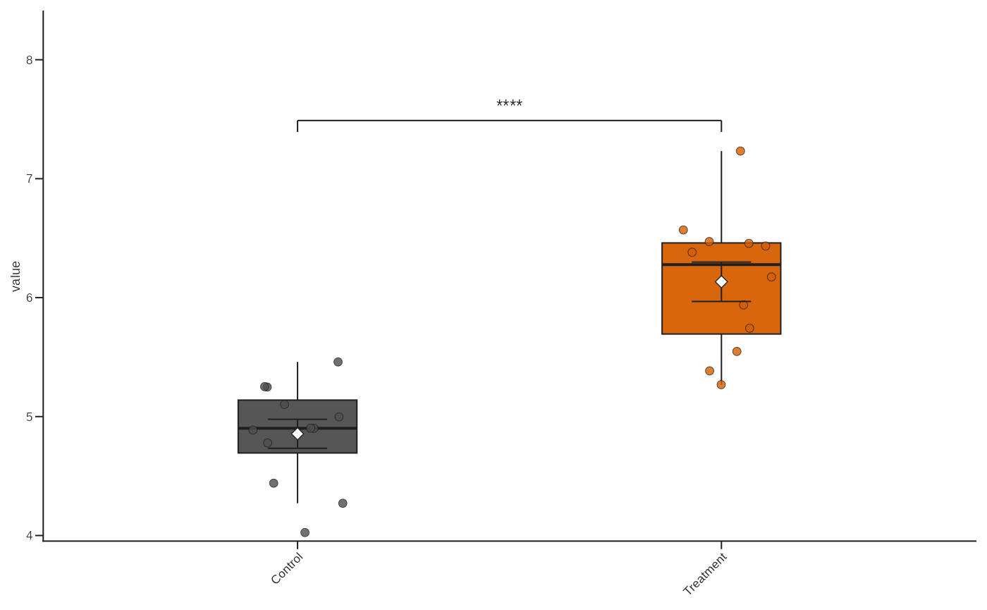
df <- data.frame(
  condition = rep(c("Control", "Treatment"), each = 12),
  value = c(rnorm(12, 5, 0.4), rnorm(12, 6.2, 0.5))
)

plot_box_paper(
  df,
  condition,
  value,
  dictionary = "default",
  show_signif = TRUE,
  comparisons = list(c("Control", "Treatment"))
)
If you prefer lower-level control, the same workflow can be built
from layer_points_paper(),
layer_summary_paper(), and
layer_signif_paper().